#load necessary libraries
library(reticulate)
library(tidyverse)
library(ggplot2)
library(dplyr)
library(purrr)
library(tibble)
library(tidyr)
library(stringr)
library(readr)
library(corrplot)
library(ggrepel)
library(dplyr)
library(ggplot2)

# Use the virtual environment created in setup.R
use_virtualenv("r-reticulate", required = TRUE)

# Import Python libraries
transformers <- import("transformers")
torch <- import("torch")7 BERT Models for Position Estimation
ManifestoBerta and IdeoBERT-it via reticulate
7.1 Setup
Load packages and data. We use reticulate to bridge R and Python, giving us access to HuggingFace transformers without leaving Positron and allowing us to write our code in the R language.
You can check if a dedicated GPU is available. If you have a dedicated GPU but it is not detected you might need to insall CUDA.
# Check PyTorch and GPU availability from R via reticulate
a <- py_run_string("
import torch
torch_version = torch.__version__
cuda_version = torch.version.cuda
cuda_available = torch.cuda.is_available()
gpu_name = torch.cuda.get_device_name(0) if cuda_available else None
")

# Print results into R console
a$torch_version  # PyTorch version
[1] "2.12.0+cu126"a$cuda_version # CUDA version PyTorch was compiled against[1] "12.6"a$cuda_available # TRUE if a GPU is detected[1] TRUEa$gpu_name # GPU model name, None if no GPU[1] "NVIDIA GeForce GTX 1050 Ti with Max-Q Design"7.2 ManifestoBerta
We will use the manifesto-project/manifestoberta-xlm-roberta-56policy-topics-sentence-2024-1-1 model, which is a BERT-based classifier fine-tuned on quasi-sentences from electoral manifestos. It classifies sentences into 56 policy categories, which can be used to construct a RILE-like index.
ManifestoBerta models are based on multilingual XLM-RoBERTa large models that were fine-tuned on all annotated statements in the Manifesto Corpus (currently more than 1.7 million annotated statements).
manifesto_pipeline <- transformers$pipeline(
  task   = "text-classification",
  model  = "manifesto-project/manifestoberta-xlm-roberta-56policy-topics-sentence-2023-1-1",
  top_k  = NULL,
  device = -1L # -1L = CPU, 0L = GPU
)
Important
Both generative models and BERT models work faster if your PC has a dedicated GPU. If you do have a dedicated GPU, make sure to replace device = -1L with device = 0L.
Even if your PC has a dedicated GPU, you might also need to install CUDA to properly use your GPU within R.
#Create a sentence
sample_sentence <- "Dobbiamo aumentare i salari minimi e proteggere i diritti dei lavoratori."

#Classify the sentence using manifestoberta
result <- manifesto_pipeline(sample_sentence)

# result is a nested R list: result[[1]] is a list of {label, score} named lists
# Convert to a tidy tibble
result_df <- result[[1]] |>
  map_dfr(as_tibble) |>
  arrange(desc(score))

print(result_df)
# A tibble: 56 × 2
label score
<chr> <dbl>
1 701 - Labour Groups: Positive 0.466
2 412 - Controlled Economy 0.461
3 408 - Economic Goals 0.0126
4 504 - Welfare State Expansion 0.00741
5 403 - Market Regulation 0.00696
6 503 - Equality: Positive 0.00689
7 706 - Non-economic Demographic Groups 0.00453
8 704 - Middle Class and Professional Groups 0.00404
9 402 - Incentives 0.00365
10 702 - Labour Groups: Negative 0.00290
# ℹ 46 more rows7.3 Classification of Investiture Speeches
The following code will load the dataset containing the sentences of the investiture speeches. We will classify only 15 sentences as an example. We will then load the dataset with the sentences already classified.
Load the data and select 15 sentences from Meloni’s speech.
#  Load data ──────────────────────────────────────────────────────────────
load("data/speeches_sentences.RData")

# Check available investiture values
unique(speeches_sentences$investituture)
[1] "BERLUSCONI IV" "MONTI" "LETTA" "RENZI"
[5] "GENTILONI" "CONTE I" "CONTE II" "DRAGHI"
[9] "MELONI" # Filter to Meloni I (adjust string to match exactly what's in your data)
speeches <- speeches_sentences |> filter(investituture == "MELONI")
# Keep sentence_id + sentence together
sentences_df <- speeches |> select(sentence_id, sentence)
# First 15 sentences for testing
sentences_df <- sentences_df[1:15, ]
sentences <- sentences_df$sentenceWe now set up the pipeline and classify the sentences. The output will be a dataset with each sentence and the probability of each category as columns.
#  Set up manifesto pipeline via reticulate ───────────────────────────────

manifesto_pipeline <- transformers$pipeline(
  "text-classification",
  model     = "manifesto-project/manifestoberta-xlm-roberta-56policy-topics-sentence-2024-1-1",
  device    = -1L,   # -1 = CPU; set to 0L for GPU
  top_k     = NULL,  # return all categories
  truncation = TRUE,
  max_length = 200L
)
Running the classification on 15 sentences is very fast, but it can take a while if you have to classify thousands of sentences.
#  Run classifier ─────────────────────────────────────────────────────────
start_time <- Sys.time()

results <- manifesto_pipeline(as.list(sentences))

end_time     <- Sys.time()
elapsed_time <- end_time - start_time
print(elapsed_time)
Time difference of 2.403214 secs
Tip
On my laptop, using the CPU, it took 3.76 to classify the sentences. With the GPU, it took only 37 seconds. If you do not have a powerful enough computer, you can use Google Colab in its free version. Here you can access a Colab notebook with a working example: ManifestoBerta Google Colab
Now we reshape the output to obtain a dataset with each row as a sentence and the probability of each category as columns.
# ── 4. Convert to long format ─────────────────────────────────────────────────
result_long <- map2_dfr(results, seq_along(results), ~ {
  tibble(
    sentence_index = .y,
    label          = map_chr(.x, "label"),
    score          = map_dbl(.x, "score")
  )
}) |>
  mutate(sentence_id = sentences_df$sentence_id[sentence_index])

# ── 5. Reshape to wide format ─────────────────────────────────────────────────
result_wide <- result_long |>
  select(sentence_id, label, score) |>
  pivot_wider(
    names_from  = label,
    values_from = score
  ) |>
  left_join(sentences_df, by = "sentence_id") |>
  select(sentence_id, sentence, everything()) |>
  arrange(sentence_id)

# ── 6. Reorder category columns by numeric prefix ────────────────────────────
category_cols         <- names(result_wide)[!names(result_wide) %in% c("sentence_id", "sentence")]
ordered_category_cols <- category_cols[order(as.integer(str_extract(category_cols, "^\\d+")))]

result_wide <- result_wide |>
  select(sentence_id, sentence, all_of(ordered_category_cols))

print(result_wide)
# A tibble: 15 × 58
sentence_id sentence 101 - Foreign Specia…¹ 102 - Foreign Specia…²
<int> <chr> <dbl> <dbl>
1 1 . 0.0156 0.0209
2 2 Grazie, Presidente. 0.0163 0.0229
3 3 Signor Presidente,… 0.0166 0.0224
4 4 Vale ovviamente a … 0.0173 0.0227
5 5 Una grande respons… 0.0174 0.0238
6 6 Sono i momenti fon… 0.0179 0.0250
7 7 Per questo io vogl… 0.0174 0.0238
8 8 Un ringraziamento … 0.0169 0.0227
9 9 Un ringraziamento … 0.0168 0.0222
10 10 E io credo che que… 0.0169 0.0227
11 11 La celerità di que… 0.0164 0.0225
12 12 E voglio per quest… 0.0176 0.0221
13 13 Si è molto ricamat… 0.0181 0.0242
14 14 Così dovrebbe esse… 0.0211 0.0250
15 15 E, tra i tanti pes… 0.0173 0.0227
# ℹ abbreviated names: ¹`101 - Foreign Special Relationships: Positive`,
# ²`102 - Foreign Special Relationships: Negative`
# ℹ 54 more variables: `103 - Anti-Imperialism` <dbl>,
# `104 - Military: Positive` <dbl>, `105 - Military: Negative` <dbl>,
# `106 - Peace` <dbl>, `107 - Internationalism: Positive` <dbl>,
# `108 - European Community/Union: Positive` <dbl>,
# `109 - Internationalism: Negative` <dbl>, …We now load the dataset with the classification of the sentences already performed.
# load the dataset
classified_sentences <-read_csv("data/speeches_sentences_classified.csv")
print(classified_sentences)
# A tibble: 17,243 × 61
doc_id2 sentence_id sentence investituture predicted_class
<chr> <dbl> <chr> <chr> <chr>
1 16_text2 1 . BERLUSCONI IV 504 - Welfare …
2 16_text2 2 Signor Presidente, onorev… BERLUSCONI IV 305 - Politica…
3 16_text2 3 Gli elettori hanno raccol… BERLUSCONI IV 305 - Politica…
4 16_text2 4 Hanno ridotto drasticamen… BERLUSCONI IV 305 - Politica…
5 16_text2 5 Il voto è stato un messag… BERLUSCONI IV 305 - Politica…
6 16_text2 6 Gli italiani hanno preso … BERLUSCONI IV 305 - Politica…
7 16_text2 7 Hanno respinto le insidio… BERLUSCONI IV 305 - Politica…
8 16_text2 8 Dividetevi - hanno detto … BERLUSCONI IV 305 - Politica…
9 16_text2 9 Combattetevi anche, ma no… BERLUSCONI IV 305 - Politica…
10 16_text2 10 Prendete democraticamente… BERLUSCONI IV 202 - Democracy
# ℹ 17,233 more rows
# ℹ 56 more variables: `101 - Foreign Special Relationships: Positive` <dbl>,
# `102 - Foreign Special Relationships: Negative` <dbl>,
# `103 - Anti-Imperialism` <dbl>, `104 - Military: Positive` <dbl>,
# `105 - Military: Negative` <dbl>, `106 - Peace` <dbl>,
# `107 - Internationalism: Positive` <dbl>,
# `108 - European Community/Union: Positive` <dbl>, …We remove some sentences and some variables that we do not need anymore.
# remove rows that have fewer than 10 characters in the sentence
classified_sentences <- classified_sentences |> filter(nchar(sentence) > 10)
print(classified_sentences)
# A tibble: 16,843 × 61
doc_id2 sentence_id sentence investituture predicted_class
<chr> <dbl> <chr> <chr> <chr>
1 16_text2 2 Signor Presidente, onorev… BERLUSCONI IV 305 - Politica…
2 16_text2 3 Gli elettori hanno raccol… BERLUSCONI IV 305 - Politica…
3 16_text2 4 Hanno ridotto drasticamen… BERLUSCONI IV 305 - Politica…
4 16_text2 5 Il voto è stato un messag… BERLUSCONI IV 305 - Politica…
5 16_text2 6 Gli italiani hanno preso … BERLUSCONI IV 305 - Politica…
6 16_text2 7 Hanno respinto le insidio… BERLUSCONI IV 305 - Politica…
7 16_text2 8 Dividetevi - hanno detto … BERLUSCONI IV 305 - Politica…
8 16_text2 9 Combattetevi anche, ma no… BERLUSCONI IV 305 - Politica…
9 16_text2 10 Prendete democraticamente… BERLUSCONI IV 202 - Democracy
10 16_text2 11 Fate funzionare le istitu… BERLUSCONI IV 305 - Politica…
# ℹ 16,833 more rows
# ℹ 56 more variables: `101 - Foreign Special Relationships: Positive` <dbl>,
# `102 - Foreign Special Relationships: Negative` <dbl>,
# `103 - Anti-Imperialism` <dbl>, `104 - Military: Positive` <dbl>,
# `105 - Military: Negative` <dbl>, `106 - Peace` <dbl>,
# `107 - Internationalism: Positive` <dbl>,
# `108 - European Community/Union: Positive` <dbl>, …#remove the column "investituture" and "sentence"
classified_sentences <- classified_sentences |> select(-investituture, -sentence)
#create doc_id3 by pasting together doc_id2 and sentence_id
classified_sentences <- classified_sentences |> mutate(doc_id3 = paste0(doc_id2, "_", sentence_id))
#remove doc_id2 and sentence_id
classified_sentences <- classified_sentences |> select(-doc_id2, -sentence_id)We load the dataset with the classification already performed and merge it with the original dataset.
#Load the dataset
read.csv("data/speeches_sentences.csv") -> speeches_sentences

#create doc_id3 by pasting together doc_id2 and sentence_id
speeches_sentences <- speeches_sentences |> mutate(doc_id3 = paste0(doc_id2, "_", sentence_id))

# leftjoin with the datasets
classified_sentences <- speeches_sentences |> left_join(classified_sentences, by = c("doc_id3"="doc_id3"))
We can now compute the RILE by speaker. The RILE is calculated by assigning each sentence to the single category with the highest probability (if that probability is above a certain threshold, e.g., 50%), and then counting how many sentences are classified as right-leaning and how many as left-leaning. The RILE score for each speaker is then calculated as (R - L) / N, where R is the number of right-leaning sentences, L is the number of left-leaning sentences, and N is the total number of sentences for that speaker.
# RILE Right categories
right_cats <- c(
  "104 - Military: Positive",
  "201 - Freedom and Human Rights",
  "203 - Constitutionalism: Positive",
  "305 - Political Authority",
  "401 - Free Market Economy",
  "402 - Incentives: Positive",
  "407 - Protectionism: Negative",
  "414 - Economic Orthodoxy",
  "505 - Welfare State Limitation",
  "601 - National Way of Life: Positive",
  "603 - Traditional Morality: Positive",
  "605 - Law and Order: Positive",
  "606 - Civic Mindedness: Positive"
)

left_cats <- c(
  "103 - Anti-Imperialism",
  "105 - Military: Negative",
  "106 - Peace",
  "107 - Internationalism: Positive",
  "403 - Market Regulation",
  "404 - Economic Planning",
  "406 - Protectionism: Positive",
  "412 - Controlled Economy",
  "413 - Nationalisation",
  "504 - Welfare State Expansion",
  "506 - Education Expansion",
  "701 - Labour Groups: Positive",
  "202 - Democracy"
)

# Filter to only columns that exist in your data
right_cats <- intersect(right_cats, colnames(classified_sentences))
left_cats  <- intersect(left_cats,  colnames(classified_sentences))
rile_cats  <- c(right_cats, left_cats)

# For each sentence: assign only the single highest RILE category if > 20
rile_df <- classified_sentences %>%
  rowwise() %>%
  mutate(
    # Get probabilities for all RILE categories for this sentence
    best_cat  = {
      vals <- c_across(all_of(rile_cats))
      names(vals) <- rile_cats
      max_val <- max(vals, na.rm = TRUE)
      if (max_val > 50) names(which.max(vals)) else NA_character_
    }
  ) %>%
  ungroup() %>%
  mutate(
    is_right = best_cat %in% right_cats,
    is_left  = best_cat %in% left_cats
  ) %>%
  group_by(doc_id2) %>%
  summarise(
    R     = sum(is_right, na.rm = TRUE),
    L     = sum(is_left,  na.rm = TRUE),
    N     = n(),
    RILE  = (R - L) / N * 100,
    .groups = "drop"
  ) %>%
  arrange(doc_id2)

print(rile_df)
# A tibble: 563 × 5
doc_id2 R L N RILE
<chr> <int> <int> <int> <dbl>
1 16_text10 10 7 28 10.7
2 16_text11 3 13 46 -21.7
3 16_text12 8 1 27 25.9
4 16_text13 7 0 28 25
5 16_text14 13 1 43 27.9
6 16_text15 14 0 38 36.8
7 16_text16 9 6 54 5.56
8 16_text17 12 3 29 31.0
9 16_text18 16 0 24 66.7
10 16_text19 6 0 9 66.7
# ℹ 553 more rowsLooking at the distribution of the RILE scores we can see that the distribution is skewd toward the right. This might be due to the fact that many sentences from the speeches are classified as “Political Authority” (category 305), which is a right-leaning category. This could be because many sentences in the speeches are about the authority of the government and the need for strong leadership, which is a common theme in political speeches.
# histogram of RILE scores
library(ggplot2)
ggplot(rile_df, aes(x = RILE)) +
  geom_histogram(binwidth = 10, fill = "steelblue", color = "white") +
  labs(title = "Distribution of RILE Scores", x = "RILE Score", y = "Frequency") +
  theme_minimal()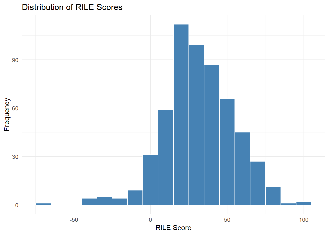
We now load the dataset with the sentences already scaled with Gemma 4, and we merge it with the dataset with the RILE scores to compare the two measures.
#load the data
scaling_results <- read_csv("data/scaling_results_gemma.csv")
#keep only doc_id2 and gemma4_scaling_mean
library(dplyr)
# keep only if sentence has more than 10 characters
scaling_results <- scaling_results |> filter(nchar(sentence) > 10)
#calculate the mean of the gemma4_scaling_mean by doc_id2

scaling_results <- scaling_results |> group_by(doc_id2) |> summarise(gemma4_scaling_mean = mean(gemma4_scaling_mean, na.rm = TRUE))
#left join scaling_results with rile_df to get the RILE scores back
scaling_results <- scaling_results |> left_join(rile_df, by = c("doc_id2" = "doc_id2"))
Now we calculate and plot the correlation between RILE and Gemma4 scores across documents.
library(ggplot2)
ggplot(scaling_results, aes(x = RILE, y = gemma4_scaling_mean)) +
  geom_point(size = 3, alpha = 0.7, colour = "steelblue") +
  geom_smooth(method = "lm", se = TRUE, colour = "tomato") +
  labs(
    x     = "ManifestoBerta RILE score",
    y     = "Gemma4 Scaling Mean",
    title = "ManifestoBerta RILE vs. Gemma4 Scaling"
  ) +
  theme_minimal()
It seems that there is a positive correlation between the two measures, but it is not perfect. This suggests that, while both models capture some similar ideological signals, they also have unique strengths and weaknesses. The RILE index is based on specific policy categories, whereas Gemma4 captures more general semantic patterns. This highlights the value of using multiple methods to triangulate political positions from text. However, the method based on ManifestoBerta might suffer from being trained on quasi-sentences from electoral manifestos, while also being subject to the same critiques of the RILE measure of ideology.
Let’s see what happens if we aggregate by party.
load("data/bow_estimates.RData")
load("data/investitutre_speeches_16_19.RData")

investitutre_speeches_16_19 <- investitutre_speeches_16_19 |> left_join(bow_estimates, by = "doc_id2")


plot_data <- investitutre_speeches_16_19 %>%
  mutate(sigla2 = case_when(
    investituture == "BERLUSCONI IV" & speaker_name_cognome == "BERLUSCONI Silvio"       ~ "BERLUSCONI (PM)",
    investituture == "MONTI"         & speaker_name_cognome == "MONTI Mario"             ~ "MONTI (PM)",
    investituture == "LETTA"         & speaker_name_cognome == "LETTA Enrico"            ~ "LETTA (PM)",
    investituture == "RENZI"         & speaker_name_cognome == "RENZI Matteo"            ~ "RENZI (PM)",
    investituture == "GENTILONI"     & speaker_name_cognome == "GENTILONI SILVERI Paolo" ~ "GENTILONI (PM)",
    investituture == "CONTE I"       & speaker_name_cognome == "CONTE Giuseppe"          ~ "CONTE I (PM)",
    investituture == "CONTE II"      & speaker_name_cognome == "CONTE Giuseppe"          ~ "CONTE II (PM)",
    investituture == "DRAGHI"        & speaker_name_cognome == "DRAGHI Mario"            ~ "DRAGHI (PM)",
    investituture == "MELONI"        & speaker_name_cognome == "MELONI Giorgia"          ~ "MELONI (PM)",
    TRUE ~ sigla
  )) %>%
  left_join(scaling_results, by = "doc_id2") %>%
  group_by(session_legislature, sigla2) %>%
  summarize(
    partymean_gemma4 = mean(gemma4_scaling_mean, na.rm = TRUE),
    partymean_rile   = mean(RILE, na.rm = TRUE),
    partymean_ws     = mean(theta_ws, na.rm = TRUE),
    partymean_wf     = mean(theta_wf, na.rm = TRUE),
    .groups = "drop"
  )

plot_data <- plot_data %>%
  mutate(label2 = paste0(sigla2, " (", session_legislature, ")"))
The two measures are only slightly correlated. The measure based on ManifestoBerta tends to cluster together parties that represent opposite ends of the ideological spectrum (e.g., PD and FDI). On the other hand, the measure based on the generative model tends to place parties on a more continuous spectrum, with higher face validity.
ggplot(plot_data, aes(x = partymean_rile, y = partymean_gemma4)) +
  geom_point(size = 3, alpha = 0.7, colour = "steelblue") +
  geom_text(aes(label = label2), vjust = -0.8, size = 3) +
  geom_smooth(method = "lm", se = TRUE, colour = "tomato") +
  theme_minimal()
We can also look at the correlation between the different measures across parties including those measured with WordScores and Wordfish.
cor_matrix <- plot_data %>%
  select(partymean_gemma4, partymean_rile, partymean_ws, partymean_wf) %>%
  cor(use = "pairwise.complete.obs")

corrplot(cor_matrix, method = "color", type = "upper", addCoef.col = "black")
7.4 Final comparison across all methods
A summary table of every method covered in the lecture series.
methods_summary <- tribble(
  ~Method,          ~Type,             ~Supervision,      ~Output,
  "Wordscores",     "BoW",             "Supervised",      "Continuous",
  "Wordfish",       "BoW",             "Unsupervised",    "Continuous",
  "LSS",            "Fixed embeddings", "Semi-supervised", "Continuous",
  "Generative LLM", "LLM (prompt)",    "Zero-shot or Few-shot",       "Continuous",
  "ManifestoBerta", "BERT classify",   "Supervised",      "RILE index",
  "IdeoBERT-it",    "BERT regress",    "Supervised",      "Continuous"
)

knitr::kable(
  methods_summary,
  caption = "Overview of text scaling methods covered in this lecture"
)| Method | Type | Supervision | Output |
|---|---|---|---|
| Wordscores | BoW | Supervised | Continuous |
| Wordfish | BoW | Unsupervised | Continuous |
| LSS | Fixed embeddings | Semi-supervised | Continuous |
| Generative LLM | LLM (prompt) | Zero-shot or Few-shot | Continuous |
| ManifestoBerta | BERT classify | Supervised | RILE index |
| IdeoBERT-it | BERT regress | Supervised | Continuous |
7.5 Other models and methods
These are only a few of the many methods available for scaling political actors along ideological dimensions using textual data. You might also consider…
7.6 Closing remarks
Text scaling is a toolbox, not a single tool. The five methods above share a common premise, political language carries ideological signal, but differ profoundly in how they extract it.
Choosing a method depends on your research question, the language of your corpus, the availability of labelled training data, and the reproducibility standards of your field.
There is no ground truth. All of these methods are operationalisations of a theoretical concept. Be transparent about your choices, report robustness checks, and let the research question drive the method, not the other way around.
The most important thing to remember is validation. It was and always will be the most important part of the process. Always validate your results against an external benchmark, and be transparent about the limitations of your chosen method. The introduction of LLMs has given us powerful new tools, but it has not changed the fundamental principles of good research design and measurement validation. Use these tools wisely, and they will open up exciting new avenues for understanding political language and ideology.
7.7 Bibliography
Burnham, Michael. 2023. “Semantic Scaling: Bayesian Ideal Point Estimates with Large Language Models.”
Lauderdale, Benjamin E., and Alexander Herzog. 2016. “Measuring Political Positions from Legislative Speech.” Political Analysis 24 (3): 374–94. https://doi.org/10.1093/pan/mpw017.
Perry, Patrick O., and Kenneth Benoit. n.d. “Scaling Text with the Class Affinity Model.”
Rheault, Ludovic, and Christopher Cochrane. 2020. “Word Embeddings for the Analysis of Ideological Placement in Parliamentary Corpora.” Political Analysis 28 (1): 112–33. https://doi.org/10.1017/pan.2019.26.
Vafa, Keyon, Suresh Naidu, and David Blei. 2020. “ACL 2020.” In, edited by Dan Jurafsky, Joyce Chai, Natalie Schluter, and Joel Tetreault, 53455357. Online: Association for Computational Linguistics. https://doi.org/10.18653/v1/2020.acl-main.475.